Overview

In part 2 of the ray tracer project we implement some more interesting materials to use in our pathtracer. We also add support for environment lighting and extend our camera with the capability of changing depth of field. I imagine in software packages such as Pixar's Renderman, which includes many shading material presets such as glass and metal, each material type is represented internally by its own particular BSDF function. In addition, Renderman's dome light is likely based on environment map lighting, with uniform sphere sampling if left to default settings and importance sampling if a texture is provided.

Part 1: Mirror and Glass Materials

The first portion of this project consisted of adding the ability to simulate mirror and glass materials. In order to replicate the behavior of light in these objects, we first needed to implement reflection and refraction of our light vectors. Because the surface normal in the object coordinate frame where BSDF calculations occur always points along the z axis, reflection is a simple negation of the xy coordinates. Refraction, however, must take into account the ratio of the indices of refraction between the exit and entrance material. This ratio varies depending on whether the outgoing ray originated within the object or outside. The rest of the coordinates follow from the spherical coordinate Snell's equations.

In order to emulate glass properly, we had to combine both reflection and refraction in the BSDF function. To do this, we needed to know the ratio of the reflection energy to the refraction energy, which we calculated using Schlick's_approximation. The algorithm is as follows: First, decide if there is internal reflection, in which case we simply reflect our outgoing light vector into our inbound vector. If there is not, we use Schlick's approximation to calculate our energy ratio and then randomly decide, with the ratio as the probability, to either reflect or refract the light ray.

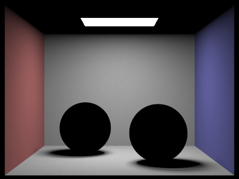
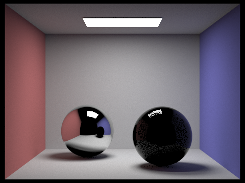
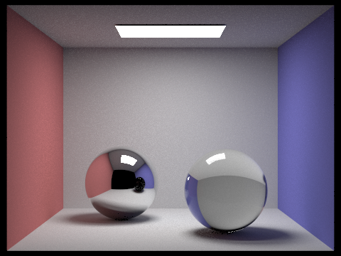
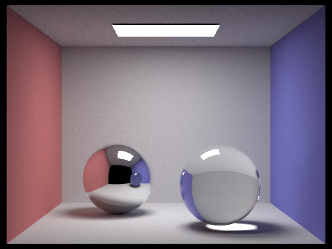
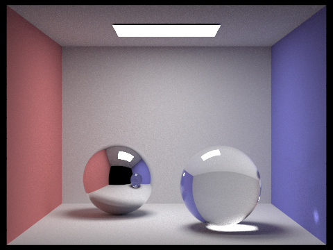
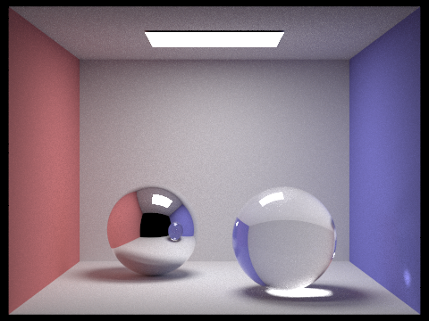
The pictures below are all of the same Cornell Box scene, containing a sphere of a mirror material on the left and a glass sphere on the right. Notice that at a maximum ray depth of 0, the spheres render as entirely black. This is because we do not permit any light bouncing, and as such light cannot be reflected off the materials. At a maximum ray depth of one, the mirror is able to reflect incoming rays and thus renders with the desired effect, but the glass has little to no internal reflection or refraction occuring, so its inside appears dark. This is resolved somewhat at a maximum depth of 2, and at a depth of 3 light is able to bounce inside the glass and re-exit, creating a white spot in the shadow of the sphere. At 4 bounces and onward, we can see a small patch of light on the bottom right corner of the blue wall, likely coming from light that reflected off the mirror sphere and refracted through the glass sphere.

Each image was generated with 1024 samples per pixel and 4 light rays.

Part 2: Microfacet Material

The next portion of the project involved implementing a "microfacet" material. Surfaces in reality are usually not perfectly smooth, instead being composed of tiny facets that have normals that are distributed about the normal of the theoretical smooth surface normal, differing by a degree determined by the roughness of the material. To implement a microfacet BRDF evaluation function, we wrote a Fresnel term to give color to the material and a normal distribution function to define how the surface normals would be distributed. In this project we used a Beckmann distribution to approximate a Gaussian (normal) probability distribution.

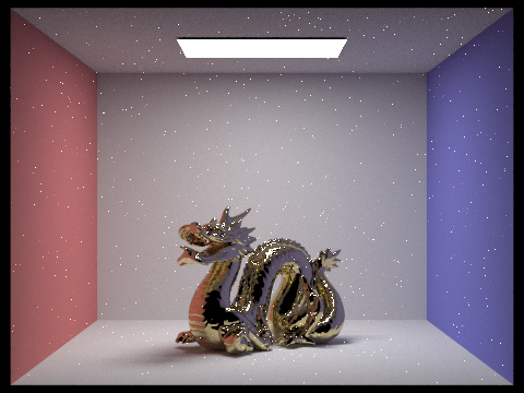
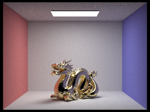
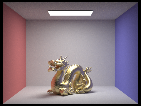
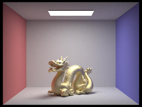
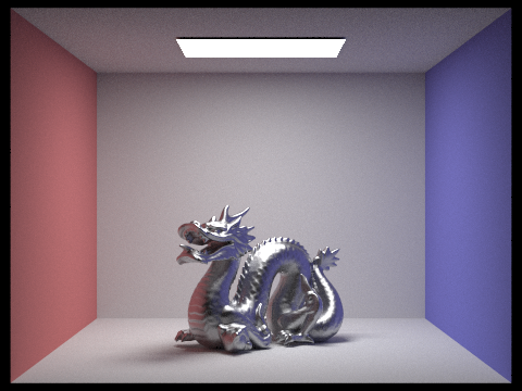
The dragon in the four images below contains a gold microfacet material. Notice as the roughness of the material increases, the dragon increases in brightness. This is due to the greater distribution of surface normals, leading to more reflections against itself. However, it also becomes less metallic and glossy, instead looking more similar to a diffuse material.

Each images was rendered with 256 samples per pixel, 4 light rays, and a maximum ray depth of 5.

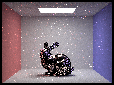
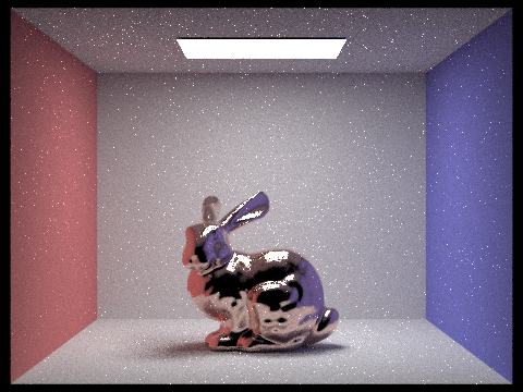
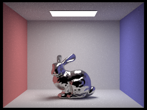
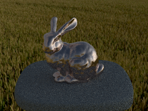
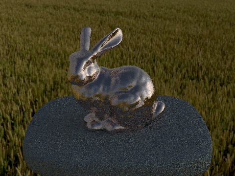
There were two approaches to sampling implemented. The first was cosine hemisphere sampling, sampling from a hemisphere with cosine-weighted points. The second approach was importance sampling. Using the Beckmann distribution from before, we use Monte Carlo integration to retrieve samples with respect to the solid angle. We do this by integrating and then inverting the probability distribution functions for the spherical coordinates theta and phi, and then combining them to calculate the pdf with respect to the solid angle.

You can see in the pictures below that importance sampling converges far faster than cosine hemisphere sampling. Overall noise, particularly on the bunny, is much lower despite using the same number of samples.

The two images below were rendered with 64 samples per pixel, 1 light ray, and a maximum of 5 light bounces.

By changing the spectrums values used in our Fresnel (color) and normal distribution terms, we can also simulate other conductor materials.

The images below were rendered with 256 samples per pixel, 4 light rays, and a maximum ray depth of 5.

Part 3: Environment Light

We implement a new light source in this part of the project, environment map lighting: an infinitely far light that provides radiance in all directions. The intensity of light in each direction is defined by a texture map, an image that also provides the 'background' of the environment.

First, we needed to get the environment image to render along with the rest of the scene. This was done by converting a camera ray's direction into an xy coordinate and then bilinearly interpolating values from the environment texture map, in a somewhat similar fashion to regular texture mapping. Initially, to simulate the effects of light from all directions, we used uniform sphere sampling to generate radiance values at various directions on the environment map.

Later, we implemented importance sampling, to bias the sampled directions towards brighter light sources. We do this in three steps. First, we calculate a prodbability distribution at each coordinate on our environment map. Then, we compute the cumulative marginal distribution and conditional distribution for that pdf. Finally, we once again use Monte Carlo integration, performing the inversion method on our marginal and conditional distribution, to retrieve an xy coordinate at which we sample and bilinearly interpolate the environment map value.

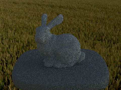
I ran into a couple issues in this part of the project. I initially had white dots appearing on my bunny, which I assumed to be noise due to uniform sphere sampling not converging quickly enough. However, despite getting the probability debug image to match the given output, the white dots continued to persist. I discovered that even if I changed my code such that the bunny would render entirely in black, it still contained the same dots, in the exact same location as well. I was able to fix this by going back to my microfacet BSDF code and updating a bound check to be <= 0 from < 0. However, for most of the environment maps aside from field, I could not figure out how to properly render either the diffuse or microfacet bunny with importance sampling, instead getting an almost entirely white bunny. I eventually realized I was incorrectly sampling from the first row of the conditional distribution, instead of the yth row based on our sample from the marginal distribution.

The pictures below were created with 4 samples per pixel and 64 light rays. The difference in noise among uniform sphere sampling and importance sampling is not nearly as noticeable as for cosine hemisphere sampling and importance sampling for the microfacet BRDF, but in the microfacet pictures you can see a slight decrease in white dots around the bunny's head.

Part 4: Depth of Field

Finally, we enable our pathtracer to simulate depth of field effects by altering our camera to simulate a thin lens (we ignore the thickness but assume that it refracts as a typical lens would). To do this, we update the rays generated from our camera with a new origin and direction. Instead of initializing all of our rays at the camera position, we take their origin to be a randomly sampled location on the thin lens. We then calculate a point of focus by intersecting our generated ray direction with the plane of focus, which is located a distance equal to the focal length away from the lens. We can get this point by calculating where the sampled coordinate intersects with the sensor plane at 1 unit away. Then, we simply multiply that by our focal distance to find our point of focus. The direction of our new generated ray then becomes the point of focus minus the point on the lens.

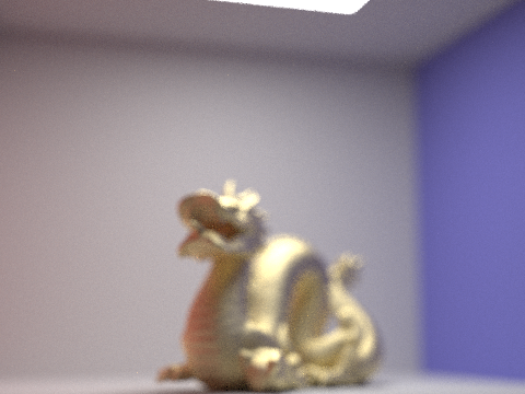
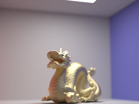
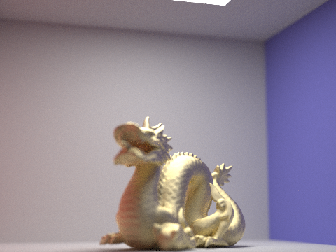
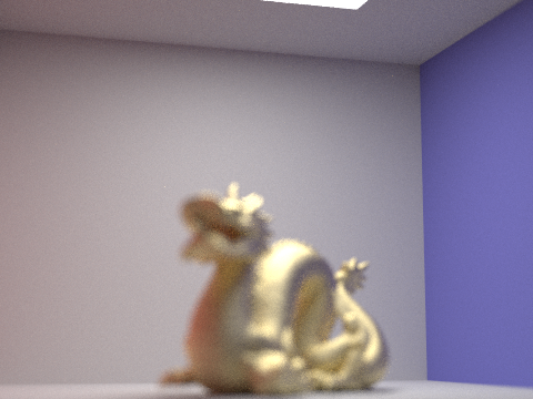
The four pictures below are the gold microfacet dragon with a roughness of 0.5. The aperture remains constant throughout each image, but the focus changes. Notice how changes in focal length lead to blurriness in various parts of the image: At a focal length of 0.25, nothing is in focus. At 0.30, only the front of the dragon enters the plane of focus. At a focal length of 0.35, the front of the dragon is no longer in focus, but the back half is. At 0.45, none of the dragon is focused anymore, but the back wall of the cornell box is.

Each picture was rendered with 256 samples per pixel, 4 light rays, a maximum ray depth of 5, and an aperture of 0.0625.

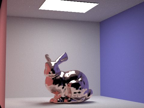
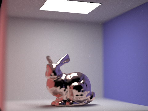
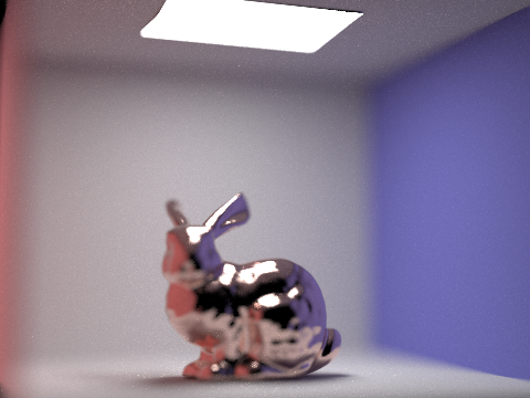
The next four pictures are of the copper microfacet bunny. Each image has the same focal length, but the aperture varies between them. At an aperture of 0, we simulate a pin-hole camera, which we have been using up to now, and everything in the frame comes into focus. At an aperture of 0.125, the walls of the cornell box start to blur while the bunny remains in focus. At higher levels, parts of the bunny begin to blur as well until only a portion of the head and upper back are in focus.

Each picture was rendered with 1024 samples per pixel, 4 light rays, a maximum ray depth of 5, and a focal length of 4.0.