In this project we implement several components of a path tracer, a system that is capable of using rays to render images and simulate lighting effects such as shadows and color bleeding. Some of the techniques involved include using an acceleration structure, the Bounding Volume Hierarchy, and Adaptive Sampling, selectively concentrating higher samples in more difficult regions of the picture, to improve our render time and image quality. It's worth mentioning that the ray tracer we build traces ray backwards, that is, we shoot rays away from the camera rather than attempt to collect light coming into it. This ensures that we do not waste computations on rays that never hit the camera (i.e. rays we never see).
For another Autodesk Maya reference, it's rather obvious that rendering must take into account some sort of path-tracing algorithm, especially to generate lighting effects. I also imagine that object detection in the viewport, that is, how the program figures out what you click on in the 3D space, is done by casting a ray from the camera to the mouse point. Then, the program tests for intersections with a BVH tree or some other acceleration structure until it can resolve an object at the click location.
|
Part 1: Ray Generation and Intersection
The first part we implemented was generating rays from the camera and testing for polygon intersections. We iterate through each pixel and generate rays through random locations within the pixel (or the center, if we are only using one sample). We then follow the ray through its path and check to see if it intersects with any triangles. To determine whether or not a ray has hit a triangle, we use the Moller Trumbore algorithm to retrieve the time of hit and barycentric coordinates of the hit point. If these variables are all within their respective bounds (a minimum and maximum time specified by our Ray struct or between (and including) 0 and 1 for our barycentric coordinates). If they are, we record in an Intersection object the time, surface normal, primitive, and bidirectional scattering distribution function (BSDF) at the hit point, and clip the ray's maximum time to the hit time so it does not continue to strike objects behind the current one.
Sphere intersection is calculated in a similar way to triangle intersection, but the quadratic formula is used to determine the times a ray enters and exits a sphere, if at all.
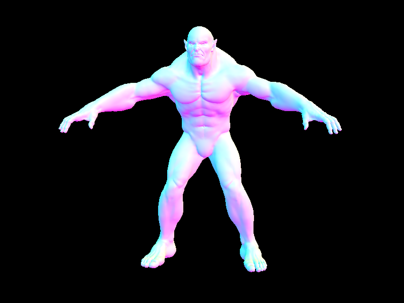
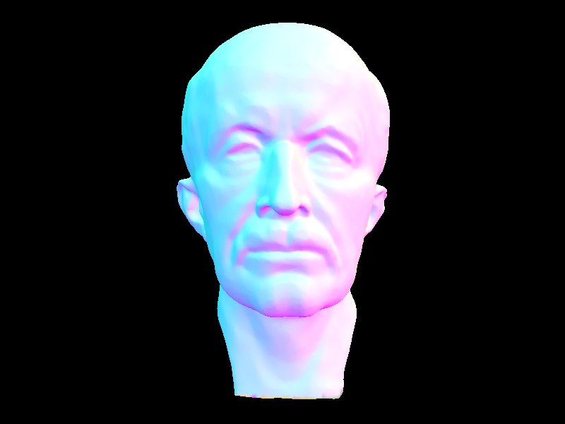
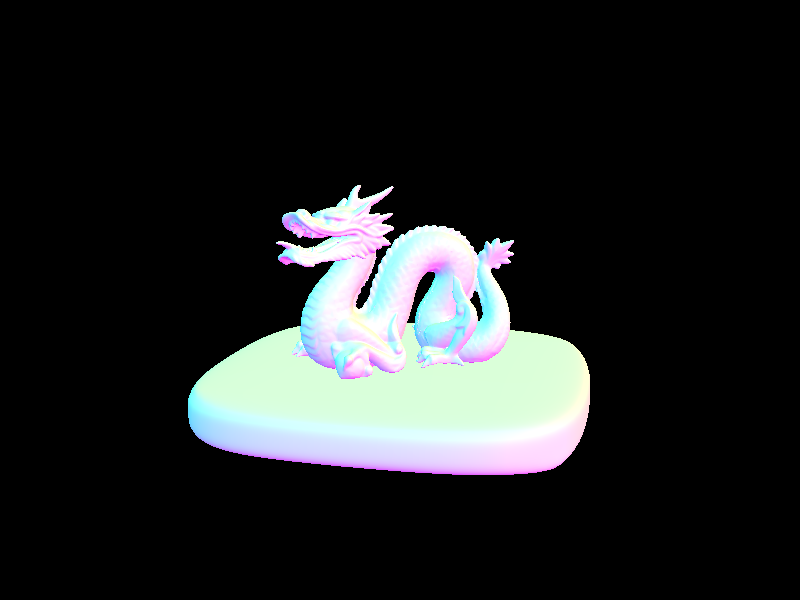
Below, the pictures are rendered using their surface normal as the shading.
|
|
|
Part 2: Bounding Volume Hierarchy
Up to now, we have been simply shooting rays at everywhere in an attempt to find an intersection. We can do better than this by using a data structure called a "Bounding Volume Hierarchy" (BVH), a special type of tree that stores information about our primitives and their bounding box, the rectangular prism that encloses all the geometry inside it. Each node contains a bounding box large enough to fit all of its children, and as you progress further down the tree the bounding box gets smaller and smaller until you reach the leaf nodes, where the actual primitive(s) are stored. We can accelerate our ray-tracing process with the BVH by testing first if a ray intersects the bounding box of a particular node. If it does not, then we know that it will not intersect any of the primitives stored in the node's children, and thus we can terminate the ray immediately instead of continuing to check for intersections.
A BVH can be built in the following fashion: Given a list of primitives, first create a bounding box that can contain the entire list and assign it to a new BVH node. If there are less primitives in our list than our preferred leaf size, we can simply assign the list to our node and terminate. If not, we want to split our primitives list into two halves. We do this by finding the maximum dimension of the bounding box, that is, the greatest length among the x, y, or z axis. We want to use the dimension of the greatest span so that our two resulting lists will encapsulate the least volume, and thus less time will be wasted on a ray that has hit empty space within the bounding box but ultimately failed to hit a primitive. After determining an axis to split on, we split the nodes based on whether their centroid coordinate on the same axis is less than or greater than the bounding box centroid coordinate. Although theoretically at this point we should have two lists of primitives, we may end up with one empty list, in which case we simply take half of one list and give it to the other. Once we retrieve our two primitive lists, we recursively assign the nodes created by calling our construction function on our two lists to the current node's left and right pointers.
Now that we have constructed a BVH tree, we can test for ray intersections. We first check if a ray has intersected the bounding box of the current node. If it does not, we know it will not intersect any of the primitives in its children, and so we can stop at that point. Otherwise, if the node is a leaf, we run through each of its primitives in order to retrieve the closest intersection (the intersection at the smallest time) and return true if we have hit anything at all. If the node is not a leaf, we recurse through both its left and right children and return true if either found a hit. It is important to note that we do not short circuit if one found a hit, rather, we attempt to explore all of the children in order to find the nearest intersection.
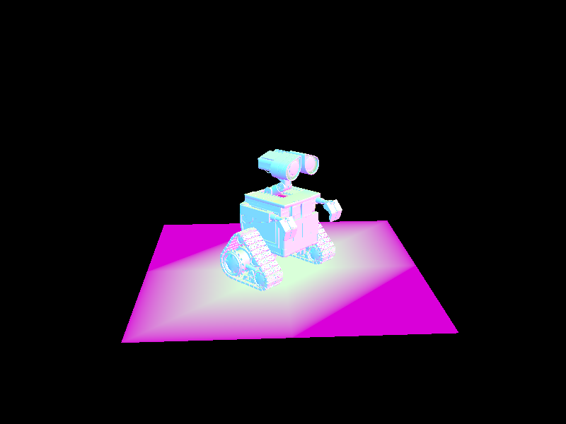
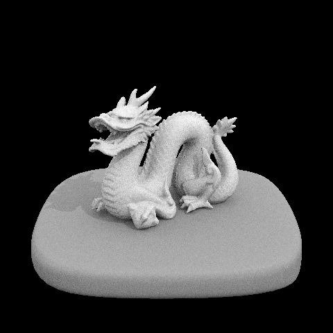
Below are images that would have taken an extraordinarily long time to render without our acceleration structure, each containing well over 50,000 primitives. Compare this to the Cornell Box coil, which at 7884 primitives is the most complicated image of the three pictured above. Thanks to the BVH tree, our render time is reduced to a few seconds.
|
|
|
|
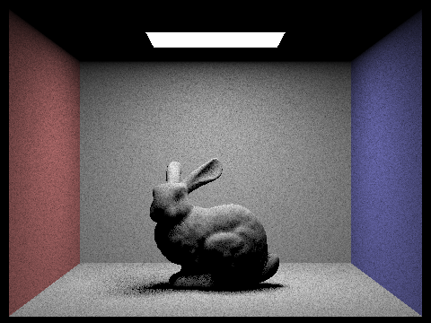
Part 3: Direct Illumination
In order to simulate the effects of direct illumination on a scene, we use the following steps. Iterating over each light in our scene, we take a number of samples at the hit point specified by a ray. At each iteration, we sample from the light and retrieve a direction vector wi from the hit point to the light source, a distance to the light, and a probability distribution function (PDF). Since wi is in world space, we convert it to object space by multiplying by a world to object transformation matrix, giving us a vector w_in. At this point we check the z coordinate of our w_in vector to determine where our sampled light point lies relative to the surface. If it is negative, we are behind the surface and can continue the loop. Otherwise, we create a ray representing the shadow with its origin at the hit point (offset by a tiny amount to account for floating point imprecision), direction wi, and a max time equal to the distance to the light. Then we test if the shadow ray does not intersect with our BVH. This ensures that we are not trying to light an area that is behind an obstacle. If we are not in a shadow, we can then accumulate the radiance from our initial sample from the light and scale it by the BSDF of the intersection primitive. We also need to divide by our PDF to correct for bias. Finally, we divide our accumulated radiance by the number of samples and add it to our total radiance spectrum.
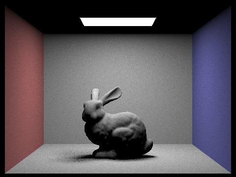
As a result you can now see shadows cast by objects in the scenes below.
|
|
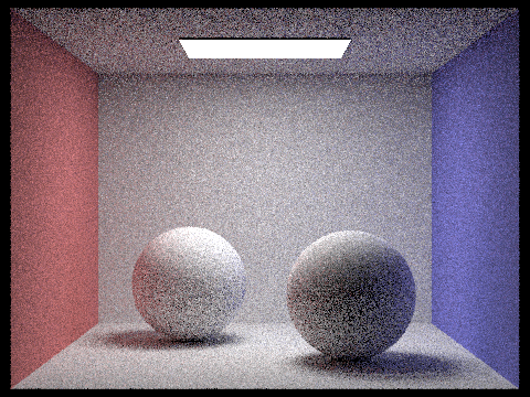
With additional light rays per pixel, you can see a substantial decrease in noise despite having only one sample per pixel.
|

|
|
|
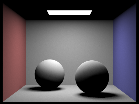
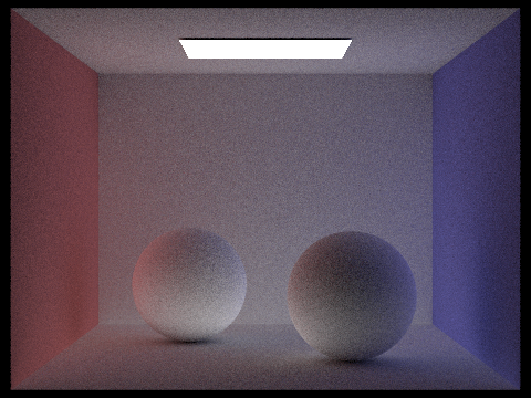
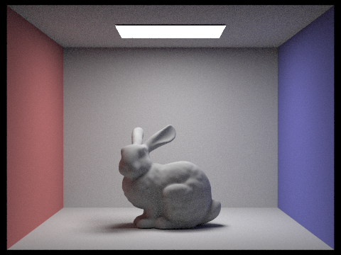
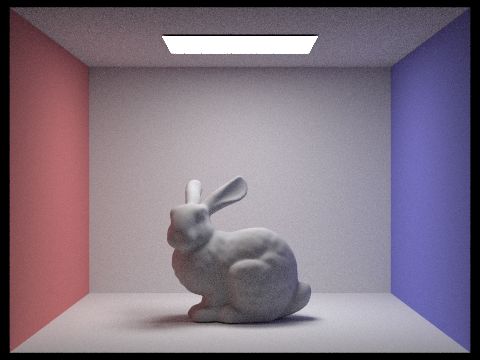
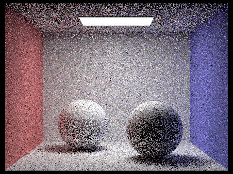
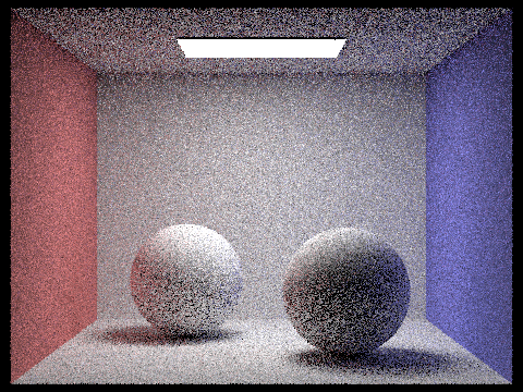
Part 4: Indirect Illumination
In order to create the effect of indirect lighting, we simulate the effects of light rays bouncing off objects. The algorithm we implement uses the reflectance of the BSDF at the intersection point as a roulette probability to determine whether or not to randomly terminate the current ray. If we decide to continue the process, we create a new ray with its origin at the hit point and its direction as the vector from the hit point to the light source. Afterwards, we set this ray's depth to be 1 less than the input ray (to ensure we will eventually terminate light bouncing) and recursively trace this ray. As such, we will calculate another direct and indirect illumination based on the bounce ray, which will also recursively calculate its own bounce rays. Once we retrieve the radiance returned to us by our initial call to ray trace, we multiply it by our BSDF and divide by our PDF value as in direct illumination. However, we also need to divide by our success probability, 1 minus the roulette probability, so as to average the radiance correctly.
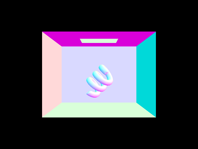
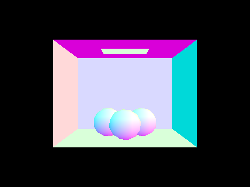
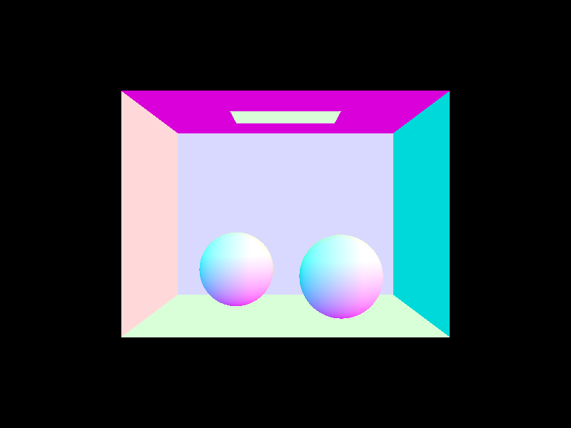
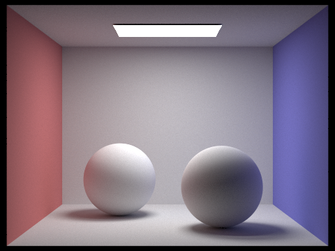
Below you can see two scenes rendered with global illumination. Notice the color bleeding in each image. In the spheres image, you can see a faint red and blue color in the top left and right corners of the box. The left sphere has a faint red on its left side and in its shadow, and the right sphere has clear tinges of blue on its side and shadow.

|

|
With no indirect illumination, you can see there is no color bleeding from the walls and the image is in fact rather dark at areas not directly in the path of the light. With no illumination directly from the source light, you can quite nicely see regions where light has bounced to give a soft light and color effect.
|
|
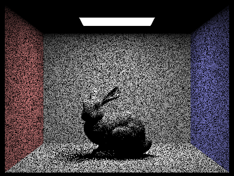
With no ray depth allowed, we get an image that is equivalent to only having direct illumination, because light is not allowed to bounce at all. Even with just one bounce allowed, you will notice the light level in the picture dramatically increases, and many places that were originally in shadow are partially lit. As we increase the allowed number of bounces, the light level continues to increase, but 100 bounces looks similar to 3. This is because light loses most of its energy within its first few bounces, and with more bounces each ray has a higher chance of being terminated.

|
|

|
|
|
|
With more samples per pixel, the image quality improves greatly. At 1024 samples, there is almost no noise in the picture.
|
|
|

|

|

|
|
Part 5: Adaptive Sampling
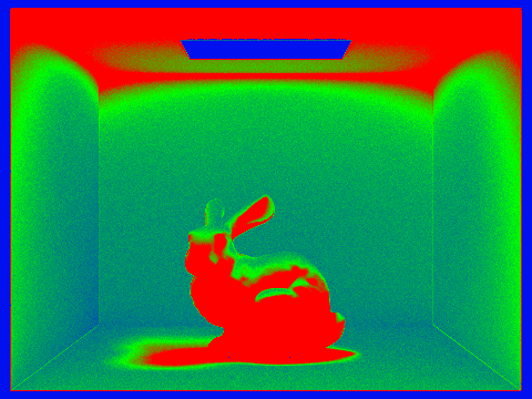
In order to eliminate noise from renders, we can increase the number of samples per pixel. However, this will significantly increase our render time if we uniformly sample every pixel with the higher sample count. Adaptive sampling is an algorithm that enables us to reduce noise while using less time and computational power than a flat increase in samples. It works by only concentrating samples in select parts of the image. Our implementation uses a statistical test to determine if a pixel's illuminance has converged or not. That is, if we are able to decide that a pixel has reached a point such that its average illuminance is within some tolerance (in our case, 5%) of its expected illuminance, then we no longer need to trace more rays for the pixel.
|
|
This technique is somewhat similar to texture mipmap levels, and the generated sampling rate image (on above right) is vaguely remniscent of a slide from an earlier lecture. Both accomplish a similar goal, increasing resolution quality while saving computational resources.